
How to Calculate Reorder Point in Excel (Formula + Free Template Logic)
The reorder point formula fits in a single Excel cell: average daily usage × lead time in days, plus safety stock. This is the exact build — which columns to lay out, the formula to type, a worked example with real numbers, and the honest limitation nobody puts in the tutorial: the spreadsheet cannot see your live stock, so the number is stale the moment usage moves.
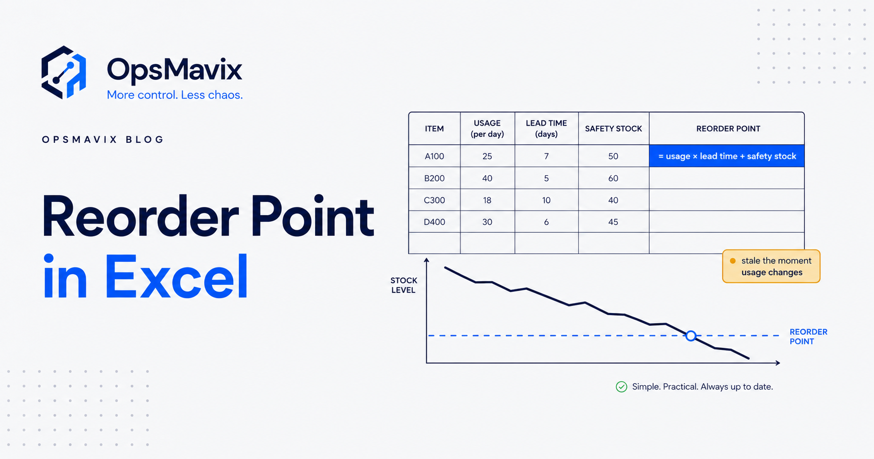
Quick summary: The reorder point formula in Excel is = average daily usage × lead time in days + safety stock, typed once and filled down a column of SKUs. Lay out one row per product with columns for average daily usage, lead time, safety stock and the calculated reorder point, then add a status column that compares live stock on hand against that reorder point. The build takes ten minutes. The catch is that a spreadsheet cannot watch your stock — the number sits there unchanged while demand drifts and stock moves, so it is only as current as the last time someone re-typed the inputs.
This is the tool-specific how-to: the exact cells, the exact formula, and a worked example you can copy. If you want the reasoning behind the numbers — why lead time matters, how the buffer is sized — that lives in the how to calculate reorder point guide, and this post assumes you just want it built in Excel.
Table of contents
- The reorder point formula, in one cell
- How to lay out the columns
- The formula typed into Excel
- A worked example with real numbers
- Adding a “reorder now?” status column
- Getting average daily usage from your sales history
- Sizing the safety stock cell honestly
- The limitation nobody puts in the tutorial
- When the spreadsheet stops being enough
- How an owned system computes the same number live
The reorder point formula, in one cell
A reorder point is the stock level at which you place a replenishment order. Hit it, and you order — because the stock you have left is just enough to cover demand while the new delivery is in transit. The formula is:
Reorder point = (average daily usage × lead time in days) + safety stock
Two parts, and they answer two different questions. The first part — average daily usage × lead time — is the lead-time demand: how many units you expect to sell or consume between placing the order and the goods landing on your shelf. The second part — safety stock — is the buffer: extra units held so that a busier-than-usual week or a late delivery does not tip you into a stockout before the replenishment arrives.
In Excel this is a single multiplication and an addition. If average daily usage is in one cell, lead time in another and safety stock in a third, the reorder point is just those three cells combined. Everything else in this post is about laying that out cleanly across a list of products and keeping the inputs honest.
How to lay out the columns
Put one product per row. The columns you need, left to right:
| Column | Header | What goes in it |
|---|---|---|
| A | SKU | Your product code |
| B | Product name | Plain-English name |
| C | Avg daily usage | Units sold/used per day |
| D | Lead time (days) | Order-to-shelf time for this item |
| E | Lead-time demand | Formula: C × D |
| F | Safety stock | Buffer units (see below) |
| G | Reorder point | Formula: E + F |
| H | Stock on hand | Current units — typed or pasted in |
| I | Reorder now? | Formula comparing H against G |
Columns E and G could be collapsed into one, but splitting out lead-time demand makes the sheet readable — you can see at a glance how much of the reorder point is “cover the wait” versus “cover the risk.” Keep the input columns (C, D, F, H) as plain numbers you edit, and the calculated columns (E, G, I) as formulas you never touch once filled down.
Freeze the top row so the headers stay visible, and format columns C to H as numbers with no decimals unless you genuinely sell in fractions.
The formula typed into Excel
Assume your first product sits on row 2, headers on row 1.
In E2 (lead-time demand):
=C2*D2
In G2 (reorder point):
=E2+F2
Or, if you skipped the separate lead-time-demand column and want the whole thing in one cell:
=C2*D2+F2
Excel follows normal order of operations, so the multiplication happens before the addition — no brackets needed, though =(C2*D2)+F2 reads more clearly and costs nothing.
Now select E2 and G2, grab the small square at the bottom-right of the selection (the fill handle), and drag down to the last product row. Excel adjusts the row references automatically — E3 becomes =C3*D3, and so on down the list. That is the entire calculator. Every product now has a live reorder point derived from its own usage, lead time and buffer.
A worked example with real numbers
Take a single SKU — a boxed filter cartridge a wholesaler sells steadily.
- Average daily usage: 40 units a day
- Lead time: 7 days from placing the order to the pallet arriving
- Safety stock: 120 units of buffer
Lead-time demand = 40 × 7 = 280 units. That is what you expect to sell while waiting for the delivery.
Reorder point = 280 + 120 = 400 units.
So when stock on hand falls to 400, you place the order. Over the next seven days you sell through roughly 280 of those, arriving at the delivery date with about 120 units — your safety stock — still on the shelf, untouched, exactly as intended. If that week ran hot and you sold 340, you still had the buffer to cover it and landed at 60 rather than zero.
In the sheet it looks like this:
| SKU | Avg daily usage | Lead time | Lead-time demand | Safety stock | Reorder point |
|---|---|---|---|---|---|
| FLT-500 | 40 | 7 | 280 | 120 | 400 |
| FLT-750 | 12 | 14 | 168 | 90 | 258 |
| VLV-200 | 5 | 21 | 105 | 60 | 165 |
Notice the second and third lines. FLT-750 sells at less than a third of the rate of FLT-500, but its reorder point is over 60% as high — because its lead time is twice as long, so it accumulates more lead-time demand per unit sold. VLV-200 barely sells, yet its three-week lead time keeps its reorder point off the floor. This is the whole reason you calculate per SKU rather than picking one round number for everything: lead time and usage pull in different directions, and a flat “reorder at 100” would leave the slow-but-slow-to-arrive lines short while overstocking the fast movers.
Adding a “reorder now?” status column
A reorder point is only useful if something checks stock against it. In Excel, column I does that with an IF:
In I2:
=IF(H2<=G2,"ORDER","OK")
Fill it down. Any row where stock on hand (H) has fallen to or below the reorder point (G) flips to “ORDER”; everything else reads “OK.” Add conditional formatting — select column I, highlight cells equal to “ORDER” in red — and the sheet becomes scannable: red rows need a purchase order raised today.
You can make it more forgiving with a “getting close” band:
=IF(H2<=G2,"ORDER",IF(H2<=G2*1.2,"WATCH","OK"))
That flags anything within 20% above the reorder point as “WATCH,” giving you a heads-up before it trips. It is a nice touch, and it exposes the real weakness at the same time: column H, stock on hand, only tells the truth if someone has just updated it. That is the crack the whole approach eventually falls through, and we will come back to it.
If you find yourself wanting a reorder up to level as well — an order-up-to quantity, not just a trigger — you have crossed into min/max inventory territory, where the reorder point is the “min” and you top back up to a defined “max.” The Excel build extends to it cleanly: add a max column and an order-quantity formula of =IF(H2<=G2, Max - H2, 0).
Getting average daily usage from your sales history
The reorder point is only as good as column C, and average daily usage is where most spreadsheets quietly lie. Typing “about 40” from memory is how lines run out.
Pull it from real sales instead. If you have a sales export with a units-sold figure per SKU over a known period, average daily usage is simply:
= total units sold in period / number of days in period
So 1,200 units of FLT-500 sold over the last 30 days gives 1200/30 = 40 a day. Use AVERAGEIF or a SUMIFS ÷ days if your export lists daily or weekly rows per SKU. The judgement call is the window: too short and one busy week distorts it; too long and you are averaging in a season that has passed. Thirty to ninety days suits most steady lines. Genuinely seasonal products need the window to track the season, which is the point where a static average stops being trustworthy at all — covered properly under demand forecasting for a small business.
Whatever window you choose, write it down in the sheet. A reorder point built on “units over the last 30 days” and never refreshed is describing a business that may no longer exist.
Sizing the safety stock cell honestly
Column F — safety stock — is the part people either fudge or over-engineer. The honest middle is to size it to the variability you actually see, not to a comfort number.
The quick, defensible approach: hold enough buffer to cover the difference between an average week and a bad one across the lead time. If FLT-500 normally sells 40 a day but spikes to 55 in a busy week, the daily gap is 15 units, and over a 7-day lead time that is roughly 105 units of exposure — which is why 120 was a sensible buffer above, not a number plucked from the air.
There is a more formal version using demand and lead-time variability (standard deviations and a service-level factor), and the full method — including the Excel-friendly version — is laid out in the safety stock calculation guide. For a spreadsheet you are maintaining by hand, the pragmatic gap-based figure above is usually the right level of effort. What matters is that safety stock is a deliberate cell you can defend, not a blanket “add 50 to everything.”
One thing to resist: do not bury safety stock inside average daily usage by inflating the usage figure. Keep the two separate. When you conflate them you lose the ability to see whether a stockout was a demand miss or a buffer that was too thin — and you will want to know which.
The limitation nobody puts in the tutorial
Here is the part the spreadsheet tutorials leave out. Your Excel reorder point is a snapshot, and it goes stale in three separate ways at once:
- Stock on hand (column H) is only true at the moment it was typed. The sheet has no connection to your actual shelves. Sell 200 units this afternoon and column H still shows this morning’s figure until a human overwrites it. The “ORDER” flag fires against a number that is already wrong.
- Average daily usage (column C) drifts. A line that sold 40 a day last quarter might be doing 60 now. The reorder point of 400 was correct for 40-a-day; at 60 a day, lead-time demand alone is 420 and you will hit a stockout before the sheet ever tells you to order, because the trigger was calibrated for a slower business.
- Lead times move. A supplier slips from 7 days to 12 and every reorder point built on 7 is now too low. Nothing in the spreadsheet knows the supplier changed.
None of these are Excel bugs. They are the nature of a spreadsheet: it computes what you last told it, and it does not watch anything. The reorder point is a live quantity pretending to be a static one. Between refreshes, the sheet is confidently displaying yesterday’s answer to today’s question — and the busier and faster-moving the business, the shorter the shelf life of that answer.
This is the honest ceiling of a reorder point in Excel. It is genuinely useful for a stable catalogue with steady demand and reliable suppliers, refreshed on a disciplined cadence. It becomes actively dangerous when the inputs move faster than the person maintaining the sheet can keep up — because then it does not just fail to help, it tells you the wrong thing with a straight face.
When the spreadsheet stops being enough
A few signals that the Excel reorder point has outgrown itself:
- You are re-typing stock on hand more than you are acting on it. The maintenance has become the job.
- Stockouts happen on lines that read “OK.” The classic tell that column H or C was stale when it mattered.
- Nobody trusts the sheet, so they eyeball the shelves anyway. The moment people route around the tool, it has stopped being a system and become a decoration.
- The list has grown past a few hundred SKUs. Manual refresh does not scale; you cannot re-derive usage for 800 lines by hand every week.
- Multiple people edit the same file. Version drift, overwritten cells, “which copy is current” — the spreadsheet’s oldest failure mode.
If two or more of those are true, the constraint is no longer the formula — you have the formula, it is right here — it is that a static file cannot keep a live quantity current. That is a structural limit, not a discipline problem, and no amount of tidier spreadsheeting fixes it. The broader version of this argument, and where the reorder point sits inside a full replenishment routine, is covered in the reorder point system.
How an owned system computes the same number live
The formula does not change when you move off the spreadsheet — average daily usage × lead time + safety stock is the same arithmetic. What changes is what watches it.
In a right-sized operations system — one built around how your business actually replenishes, sitting in that gap where you are too messy for spreadsheets but not ready for a full ERP — the three inputs are no longer typed by hand:
- Stock on hand updates itself as sales, receipts and adjustments happen, so the reorder point is always compared against the real current figure, not a morning snapshot.
- Average daily usage is recomputed on a rolling window from live sales, per SKU, so the trigger tracks the business as it speeds up or slows down instead of freezing at last quarter’s rate.
- Lead times can be pulled from actual receipt history — the real gap between order and delivery per supplier — rather than a hopeful number in column D.
- The reorder check runs continuously, so instead of you scanning for red rows, the system raises the flag the moment a SKU crosses its own line, and it does it across the whole catalogue at once.
The point is not that Excel is wrong. The point is that Excel makes the reorder point a thing you maintain, and an owned system makes it a thing that maintains itself — the same number, watched live per SKU, so it is current at the moment you need to act on it rather than at the moment someone last had time to update a file. That is the difference between a calculator and a control. If you want to see what that looks like without the spreadsheet in the middle, the fully automated inventory system piece walks through it.
The short version
Build it in Excel today: one row per SKU, columns for average daily usage, lead time, safety stock, a =C2*D2+F2 reorder point, and an =IF(H2<=G2,"ORDER","OK") status. Pull usage from real sales, size safety stock to the variability you actually see, and refresh the inputs on a disciplined cadence. Then be honest about the ceiling: the sheet computes what you last told it and watches nothing, so the faster your business moves, the sooner its answer goes stale. The formula is not the hard part — keeping the inputs live is, and that is exactly the job a spreadsheet cannot do.